Document Deduplication with Locality Sensitive Hashing
Applications utilising Natural Language Processing (NLP) have recently gained alot of traction partly due to advances in artificial neural networks. One especially tricky problem for NLP however begins before you even get to the “processing” part, namely the deduplication of the incoming document stream.
Online platforms such as recommender systems as well as comment forums and user feedback systems all face the problem of detecting which documents are duplicates of each other. As many NLP tasks tend to be computationally expensive it is desirable to only apply those processes to new documents. The class label or action taken upon seeing a duplicate document is likely the same as that for the original.
It is also important to keep duplicates out of your training data to prevent them from unfairly biasing the trained model. The prevalence of certain document features and their relation to the task at hand can be severly biased by multiple duplicate entried of the same document or documents. Obviously storing duplicate documents in your backend system is also a waste of resources.
How do you determine if a document is a duplicate or more importantly a near duplicate? Ideally the method of deduplication would work online and have predictable resource requirements. As always the faster the model works the better, especially at decoding time, that is when the model is being applied to new unseen instances.
I will first outline a simple and effective way of detecting near duplicates: character shingles and Jaccard similarity. I’ll then discuss ways of making that process computationally feasible using locality sensitive hashing with minhash. Before we get to the nitty gritty of detecting near duplicates let’s first consider where duplicate documents come from and what it means for an article to be a near duplicate.
Document Similarity and Duplicates
When we talk about similar documents we usually mean documents that are semantically related, for instance two different news articles about the same event. There are a number of ways for determining the semantic relatedness of documents, for instance Latent Dirichlet Allocation (LDA) or neural language models. The semantic relatedness however is not what I mean by near duplicate documents. Near duplicates are not two different takes on one event but explicitly the same article duplicated across different channels. Near duplicate documents are of course also semantically related but it is important to make the distinction.
Semantic similarity of documents is relatively easy for humans to detect but extremely difficult to do algorithmically, especially for longer documents. The main area of research here is distributional semantics, specifically distributional composition. In short distributional composition is about how the semantics of individual words should be composed together to form a semantic represenatation of larger pieces of text like sentences and documents, neural language models are one example of this.
Distributional composition is an active area of research and I won’t focus on it here, if you’re interested you’ll probably want to look at the publications coming out of ACL, TACL, EMLNP and NIPS. The second and much simpler kind of similarity is character based similarity, which quite simply measures the character overlap between two sentences or documents.
Where Do Duplicates Come From?
Duplicates are often produced in news media when a content producer like Reuters or the Associated Press distributes an article to a number publishers. Each publisher will typically add a paragraph or a footer making each copy slightly different from each other. A web crawler that monitors the sites of the individual publishers will see many near duplicate articles as each copy was essentially written by Reuters and only slightly modified by the other publishers.
Duplicate news articles also tend to come in the form of updated news stories. Typically publishers will use an older version of the article and add a paragraph or two in the beginning with the new updated information, the rest of the article typically remains unchanged.
Near duplicates can also appear in user feedback systems in the event of a system or process failure. The feedback system will suddenly log a number of a documents created by different users that all look roughly similar. Product or service review sites can also experience this, possibly in the form of spam reviews being posted by automated systems.
Another interesting data set that potentially contains duplicates is the recently released Quora Question Pairs dataset. Here the aim is specifically to find questions that are semantically the same, but often those questions are just slighty paraphrased ones.
Paul Jaccard and Roofing
Now that we know where near duplicated come from and how they differ from documents that are semantically related, let’s outline how one could go about detecting them.
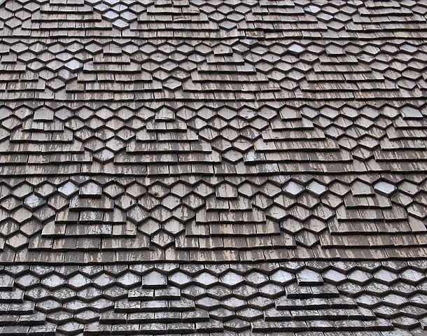
The method relies on two simple concepts, character shingles and the Jaccard similarity. ‘Shingle’ is a term that comes from roofing and refers to partially overlapping pieces of clay, stone, wood, asphalt or some such bits of roofing material.
The idea for character shingles is similar, create a document representation of consecutive overlapping character n-grams from each document. “Cat sat on the mat”, when 4-shingled becomes ('The ', 'he c', 'e ca', ' cat', … ,'at.'). Notice that punctuation and whitespace are all part of the process. This represenatation preserves word order, to some extent, and allows comparing documents based on the sets of character shingles. The similarity of those documents can then simply be defined as the Jaccard similarity of the two sets of shingles; the number of elements (shingles) they have in common as a proportion of the combined size of the two sets, or the size of the intersection divided by the size of the union.
For two dummy sentences let’s see how the length of the character shingle effects the similarity of the documents. We’ll use python’s matplotlib and seaborn libraries to plot the similarities.
%matplotlib inline
from matplotlib import pyplot as plt
import seaborn as sns # makes the graph prettier

s1 = "The cat sat on the mat."
s2 = "The red cat sat on the mat."

similarities = []
for shingle_size in range(2, 6):
    shingles1 = set([s1[max(0, i - shingle_size):i] for i in range(shingle_size, len(s1) + 1)])
    shingles2 = set([s2[max(0, i - shingle_size):i] for i in range(shingle_size, len(s2) + 1)])
    jaccard = len(shingles1 & shingles2) / len(shingles1 | shingles2)
    similarities.append(jaccard)

_ = plt.bar([2,3,4,5], similarities, width=0.25)
_ = plt.xlabel('Jaccard Similarity')
_ = plt.ylabel('Shingle Size')
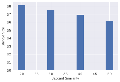
Leaving aside the discussion of whether a red cat sitting on a mat is in fact a “duplicate” of a cat sitting on a mat, what it means for something to be red or indeed a cat, I will declare those two “documents” as duplicates of each other. With a shingle size of 2 we get a similarity of ~0.81 (or 81%) and with a shingle size of 5 we get a similarity of ~0.62 or 62%.
The size of the shingle clearly has an impact on the effectiveness of this approach, one should however bear in mind that the two “documents” are very short especially in comparison to a shingle size of 5. The average word length in those two documents is just under 3, so a shingle size of 5 is actually comparing chunks that are bigger than single words. For longer documents that better reflect actual language usage the shingling will produce much more reasonable outputs. There are of course cases where this kind of character similarity will fail, let’s explore those corner cases in a bit more detail.
Where Character Similarity Fails
It is not difficult to come up with sentences that are semantically the same but share only a small proportion of their shingles, for example: “What’s the flight time from Berlin to Helsinki” and “How long does it take to fly from Berlin to Helsinki” are semantically exactly the same but have very few words or character n-grams in common. On the other hand “What’s the flight time from Berlin to Helsinki” and “What’s the flight time from Berlin to Oulu” are semantically not the same but have a large character overlap.
s1 = "what's the flight time from Berlin to Helsinki?"
s2 = "how long does it take to fly from Berlin to Helsinki?"

shingles1 = set([s1[max(0, i-4):i] for i in range(4, len(s1) + 1)])
shingles2 = set([s2[max(0, i-4):i] for i in range(4, len(s2) + 1)])

len(shingles1 & shingles2) / len(shingles1 | shingles2)
0.30985915492957744
s1 = "what's the flight time from Berlin to Helsinki?"
s2 = "what's the flight time from Berlin to Oulu?"

shingles1 = set([s1[max(0, i-4):i] for i in range(4, len(s1) + 1)])
shingles2 = set([s2[max(0, i-4):i] for i in range(4, len(s2) + 1)])

len(shingles1 & shingles2) / len(shingles1 | shingles2)
0.7142857142857143
These two are again simple example sentences but it is important to understand where the limits of any particular method or technology lie. The initial exploration has already revealed a critical relationship between the length of the document and the length of the character shingle, suggesting that the method might not work so well for data that contains a lot of short one sentence documents, for instance tweets. Equally it’s unlikely to work all that well for rephrased sentences or documents, the semantics of rephrased or summarised information should not change but the character representation will.
This should all be fine however, as we’ve already defined the task to be about finding near duplicate documents not semantically similar ones, for document collections with longer documents this method should work very well.
A Real World Example
Deduplicating the Reuters RCV1 corpus
The Reuters Corpus, Volume 1 (RCV1) corpus is a commonly used resource for various NLP tasks, especially document classification. It was made available in 2000 by Reuters Ltd. and consists of ~800,000 english language news stories collected between August 20th 1996 and August 19th 1997 from the Reuters news wire.
I’ve preprocessed the corpus so that it is all in a single file, one line per document. Each line has the format:
ITEMID<TAB>HEADLINE<SPACE>TEXT
!wc -l /usr/local/scratch/data/rcv1/headline.text.txt
806791 /usr/local/scratch/data/rcv1/headline.text.txt
!head -1 /usr/local/scratch/data/rcv1/headline.text.txt | cut -c -100
2286 Recovery excitement brings Mexican markets to life. Emerging evidence that Mexico's economy wa
Some duplicate items are present in the corpus so let’s see what happens when we apply the shingling with Jaccard similarity method to the corpus.
import itertools

# from lsh import lsh, minhash # https://github.com/mattilyra/lsh

# a pure python shingling function that will be used in comparing
# LSH to true Jaccard similarities
def get_shingles(text, char_ngram=5):
    """Create a set of overlapping character n-grams.

    Only full length character n-grams are created, that is the first character
    n-gram is the first `char_ngram` characters from text, no padding is applied.

    Each n-gram is spaced exactly one character apart.

    Parameters
    ----------

    text: str
        The string from which the character n-grams are created.

    char_ngram: int (default 5)
        Length of each character n-gram.
    """
    return set(text[head:head + char_ngram] for head in range(0, len(text) - char_ngram))


def jaccard(set_a, set_b):
    """Jaccard similarity of two sets.

    The Jaccard similarity is defined as the size of the intersection divided by
    the size of the union of the two sets.

    Parameters
    ---------
    set_a: set
        Set of arbitrary objects.

    set_b: set
        Set of arbitrary objects.
    """
    intersection = set_a & set_b
    union = set_a | set_b
    return len(intersection) / len(union)
Let’s first try this pure python implementation on the first 500 documents.
shingles = []
with open('/usr/local/scratch/data/rcv1/headline.text.txt', 'r') as fh:
    for i_line, line in enumerate(fh):
        if i_line > 500:
            break
        document_id, article_text = line.split('\t', maxsplit=1)
        shingles.append(get_shingles(article_text.lower()))
duplicates = []
for i_doc in range(len(shingles)):
    for j_doc in range(i_doc + 1, len(shingles)):
        jaccard_similarity = jaccard(shingles[i_doc], shingles[j_doc])
        is_duplicate = jaccard_similarity >= 0.75
        if is_duplicate:
            duplicates.append((i_doc, j_doc, jaccard_similarity))
len(duplicates)
36
import pandas as pd

pd.DataFrame(duplicates, columns=['Document ID', 'Document ID', 'Jaccard Similarity']).head(n=10)
| Document ID | Document ID | Jaccard Similarity | |
|---|---|---|---|
| 0 | 2 | 3 | 1.00 |
| 1 | 13 | 160 | 1.00 |
| 2 | 19 | 180 | 0.88 |
| 3 | 22 | 176 | 0.91 |
| 4 | 25 | 77 | 0.80 |
| 5 | 29 | 69 | 0.75 |
| 6 | 31 | 32 | 1.00 |
| 7 | 47 | 190 | 1.00 |
| 8 | 48 | 49 | 1.00 |
| 9 | 48 | 195 | 0.84 |
If we look at the documents themselves we can easily see how accurately the algorithm is detecting duplicate documents. Let’s see what documents 2 and 3 look like. We don’t really care what the first 6 character are as those are just the document ID and a <TAB>.
!head -4 /usr/local/scratch/data/rcv1/headline.text.txt | tail -2 | cut -c 6-350
CompuServe reports loss, cutting work force.  CompuServe Corp. Tuesday reported a surprisingly large $29.6 million fiscal first-quarter loss, blaming a decline in the number of subscribers to the No. 2 online service and spending on a new family-oriented service and improvements. CompuServe predicted a second-quarter loss but said earnings wou
CompuServe reports loss, cutting work force.  CompuServe Corp. Tuesday reported a surprisingly large $29.6 million fiscal first-quarter loss, blaming a decline in the number of subscribers to the No. 2 online service and spending on a new family-oriented service and improvements. CompuServe predicted a second-quarter loss but said earnings wou
Judging by the first 350 characters of the articles it would seem that the documents are indeed exact duplicates. Let’s see what near duplicates look like, this time we’ll take documents 25 and 77 which have been assigned a similarity score of 0.80 or 80%.
!head -26 /usr/local/scratch/data/rcv1/headline.text.txt | tail -1 | cut -c 6-450
Lloyd's chief undergoes U.S. grilling. Lloyd's of London chief executive Ron Sandler on Tuesday faced a three-hour grilling in a crucial United States court case, which threatens at the last minute to upset a recovery plan for the 300-year-old insurance market. Tens of thousands of investors in Lloyd's worldwide are anxiously awaiting the outcome of the case in Virginia, where U.S. investors (Names) have applied for an injunction to stop th
!head -78 /usr/local/scratch/data/rcv1/headline.text.txt | tail -1 | cut -c 6-450
Lloyd's braced for crucial U.S. court case ruling. Lloyd's of London was braced on Tuesday for a possible ruling in a crucial United States court case, which threatens at the last minute to upset a recovery plan for the 300-year-old insurance market. Tens of thousands of investors in Lloyd's worldwide are anxiously awaiting the outcome of the case in Virginia, where U.S. investors (Names) have applied for an injunction to stop the recovery
There are more differences between the two, but they are essentially talking about the exact same thing. A few sentences have been paraphrased but otherwise the documents look identical. So the method seems to be working.
len(duplicates), (len(duplicates) / 500) * 100
(36, 7.199999999999999)
Approximately 7 percent of the first 500 documents are in fact duplicates, that translates to about 57,000 duplicate documents in the relatively small 800,000 document dataset overall. The problem is that finding those duplicates took quite a long time as computing the Jaccard similarity of the documents requires comparing every document to every other document, this approach is clearly not scalable. This is where Locality Sensitive Hashing with minhash comes in.
Locality Sensitive Hashing
Locality Sensitive Hashing (LSH) is a generic hashing technique that aims, as the name suggests, to preserve the local relations of the data while significantly reducing the dimensionality of the dataset. It can be used for computing the Jaccard similarities of elements as well as computing the cosine similarity depending on exactly which hashing function is selected, more on this later.
LSH is a slightly strange hashing technique as it tries to ensure hash collisions for similar items, something that hashing algorithms usually try to avoid. The overall aim is to reduce the number of comparisons needed to find similar items, the hash collisions come in handy here as similar documents have a high probability of having the same hash value. The hash values can be treated as an address for a bucket that contains likely duplicates, this reduces the number of comparisons needed as only the documents contained in a bucket, not every other document, need to be looked at to find the real duplicates.
Locality sensitive hashing is great but it’s not quite enough on its own. It would also be great if we could predict the computational requirements of the process overall. As it stands each document is shingled into some number of shingles, the exact number of which depends on the length of the document and the size of the shingle. Each document therefore has an unpredictable memory footprint, ideally we’d have a document representation whose size is independent of the length of the document without changing the semantics of document similarity.
This is where minhash comes in, it’s a specific hash function that has some desirable properties for this use case. Namely, it turns out that the probability of a hash collision for a minhash is exactly the Jaccard similarity of two sets. This can be seen by considering the two sets of shingles as a matrix. For two dummy documents the shingles could be represented as the table below (the zeros and ones indicate if a shingle is present in the document or not). For this discussion it doesn’t matter what the actual shingles are, but notice that the Jaccard similarity of the documents is 2/5, that is 2 out of 5 shingles (shingle IDs 2 and 4) are shared between the documents.
| Document Shingles | |||
|---|---|---|---|
| row | shingle ID | Doc 1 | Doc 2 |
| 1 | 1 | 0 | 1 |
| 2 | 2 | 1 | 1 |
| 3 | 3 | 0 | 1 |
| 4 | 4 | 1 | 1 |
| 5 | 5 | 1 | 0 |
| 6 | 6 | 0 | 0 |
The minhash corresponds to a random permutation of the rows and gives back the row number where the first non zero entry is found. For the above table the minhash for documents one and two would thus be 2 and 1 respectively - meaning that the documents are not similar. The above table however is just one ordering of the shingles of each document. A different random permutation of the rows will give a different minhash, in this case 2 and 2, making the documents similar.
| Document Shingles | |||
|---|---|---|---|
| row | shingle ID | Doc 1 | Doc 2 |
| 1 | 6 | 0 | 0 |
| 2 | 2 | 1 | 1 |
| 3 | 3 | 0 | 1 |
| 4 | 1 | 0 | 1 |
| 5 | 4 | 1 | 1 |
| 6 | 5 | 1 | 0 |
A random permutation of the rows can produce any of 6! == 720 (factorial) different orderings. However we only care about the orderings for which the two columns have the same lowest row number with a 1, that is shingle ID . Since the rows with zeros on them don’t count, there are 5 rows with a one on it in any column, and two rows with a 1 in both columns. All a random permutation can therefore do is put two out of the five rows in the lowest row number, in other words produce a hash collision with a probability 2/5.
The above explanation follows Chapter 3 of Mining Massive Datasets (Leskovec, Rajaraman and Ullman). An in depth explanation for why and how minhash works is provided there along with other interesting hash functions.
Using minhash we can create a fixed length fingerprint from each document, where each item in the fingerprint is a different random permutation of the rows. The longer the fingerprint the higher the likelihood that duplicate documents have a hash collision for at least one of the permutations. You’re not guaranteed to get a collision, but you get to control the memory requirements of your document deduplication algorithm. The graph below shows the relation between the actual Jaccard similarity of a pair of documents and the probability it will be discovered for a few different parameter settings of LSH.
df = pd.DataFrame(data=[(2, 50), (50, 2), (10, 10), (5, 20), (20, 5)], columns=['pieces', 'size'])
df['hashes'] = df['pieces'] * df['size']
for pr in np.linspace(0, 1, 200):
    df[pr] = 1 - (1 - pr**df['size']) ** df['pieces']

df = pd.pivot_table(df, index=['hashes', 'pieces', 'size'])

ax = df.T.plot(figsize=(10, 7), title='Probability of LSH finding a candidate pair');
plt.ylabel('p(candidate | Jaccad)');
plt.xlabel('Jaccard similarity');
plt.legend(list(df.loc[ix[100]].index),
           bbox_to_anchor=(1., 1, 1., 0), loc='upper left', fontsize=12,
           ncol=1, borderaxespad=0., title='Each line shows the\nfingerprint chopped\ninto (pieces, size)\n');
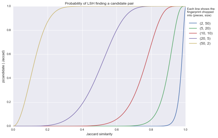
The figure shows the probability that LSH with minhash will “find” a pair of similar documents (y-axis) given the Jaccard similarity (x-axis) of those documents for different settings for LSH. Each of the five lines correspond to different settings, the number of hashes is always 100 so we’re just changing the number of pieces to chop each fingerprint into (and the size of those pieces, although that becomes determined by setting the number of hashes).
Creating just two pieces with 50 rows each - that is two localities, each with a size of 50 minhashes - yields an LSH model (the blue line) that tries really really hard not to find documents to be similar. This LSH model will find 80% of documents whose actual Jaccard similarity is over 95%. Documents whose Jaccard similarity is 80% will hardly ever be found to be similar.
Creating 5 pieces with 20 rows (the green line) each is slightly more relaxed. The above graph should give you a pretty good idea how to set the parameters for your use case so that you can be reasonably certain that LSH will generate acceptable candidate pairs.
Now let’s return to the RCV1 corpus and see how well we can expect LSH to work. First let’s just see how many candidate pairs different settings for LSH produce.
def candidate_duplicates(document_feed, char_ngram=5, seeds=100, bands=5, hashbytes=4):
    char_ngram = 5
    sims = []
    hasher = minhash.MinHasher(seeds=seeds, char_ngram=char_ngram, hashbytes=hashbytes)
    if seeds % bands != 0:
	    raise ValueError('Seeds has to be a multiple of bands. {} % {} != 0'.format(seeds, bands))

    lshcache = cache.Cache(num_bands=bands, hasher=hasher)
    for i_line, line in enumerate(document_feed):
	    line = line.decode('utf8')
	    docid, headline_text = line.split('\t', 1)
	    fingerprint = hasher.fingerprint(headline_text.encode('utf8'))

	    # in addition to storing the fingerpring store the line
	    # number and document ID to help analysis later on
	    lshcache.add_fingerprint(fingerprint, doc_id=(i_line, docid))

    candidate_pairs = set()
    for b in lshcache.bins:
	    for bucket_id in b:
		    if len(b[bucket_id]) > 1:
			    pairs_ = set(itertools.combinations(b[bucket_id], r=2))
			    candidate_pairs.update(pairs_)

    return candidate_pairs


num_candidates = []
bands = [2, 5, 10, 20]
for num_bands in bands:
    with open('/usr/local/scratch/data/rcv1/headline.text.txt', 'rb') as fh:
	    feed = itertools.islice(fh, 1000)
	    candidates = candidate_duplicates(feed, char_ngram=5, seeds=100, bands=num_bands, hashbytes=4)
	    num_candidates.append(len(candidates))

fig, ax = plt.subplots(figsize=(8, 6))
plt.bar(bands, num_candidates, align='center');
plt.title('Number of candidate duplicate pairs found by LSH using 100 minhash fingerprint.');
plt.xlabel('Number of bands');
plt.ylabel('Number of candidate duplicates');
plt.xticks(bands, bands);
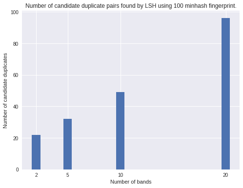
The more promiscuous version (20 bands per fingerprint) finds many more candidate pairs than the conservative 2 bands model. The first implication of this difference is that it leads to you having to do more comparisons to find the real duplicates. Let’s see what that looks like in practice.
lines = []
with open('/usr/local/scratch/data/rcv1/headline.text.txt', 'rb') as fh:
    # read the first 1000 lines into memory so we can compare them
    for line in itertools.islice(fh, 1000):
        lines.append(line.decode('utf8'))

    # reset file pointer and do LSH
    fh.seek(0)
    feed = itertools.islice(fh, 1000)
    candidates = candidate_duplicates(feed, char_ngram=5, seeds=100, bands=20, hashbytes=4)

# go over all the generated candidates comparing their similarities
similarities = []
for ((line_a, docid_a), (line_b, docid_b)) in candidates:
    doc_a, doc_b = lines[line_a], lines[line_b]
    shingles_a = shingles(lines[line_a])
    shingles_b = shingles(lines[line_b])

    jaccard_sim = jaccard(shingles_a, shingles_b)
    fingerprint_a = set(hasher.fingerprint(doc_a.encode('utf8')))
    fingerprint_b = set(hasher.fingerprint(doc_b.encode('utf8')))
    minhash_sim = len(fingerprint_a & fingerprint_b) / len(fingerprint_a | fingerprint_b)
    similarities.append((docid_a, docid_b, jaccard_sim, minhash_sim))
import random

print('There are {} candidate duplicates in total'.format(len(candidates)))
random.sample(similarities, k=15)
[('2317', '2293', 0.6090381426202321, 0.4492753623188406),
 ('2544', '2403', 0.8514745308310991, 0.7094017094017094),
 ('2742', '2387', 0.6901698404529079, 0.4925373134328358),
 ('2306', '2940', 0.4451428571428571, 0.26582278481012656),
 ('2506', '2507', 0.996265172735761, 1.0),
 ('2335', '2536', 0.8379651436646255, 0.7241379310344828),
 ('2361', '2315', 0.7490176817288802, 0.5748031496062992),
 ('2311', '2372', 0.7974055703929798, 0.7241379310344828),
 ('2302', '2971', 0.576, 0.5151515151515151),
 ('2910', '2857', 0.9893048128342246, 0.941747572815534),
 ('2336', '2338', 0.9870317002881844, 0.9801980198019802),
 ('2312', '2303', 0.6593059936908517, 0.45985401459854014),
 ('2486', '2875', 0.6749619095987811, 0.5037593984962406),
 ('2323', '2451', 0.7245482591449978, 0.5267175572519084),
 ('3256', '3186', 0.3084023668639053, 0.11731843575418995)]
So LSH with 20 bands indeed finds a lot of candidate duplicates (111 out of 1000), some of which - for instance (3256, 3186) above - are not all that similar. Let’s see how many LSH missed given some similarity threshold.
sims_all = np.zeros((1000, 1000), dtype=np.float64)
for i, line in enumerate(lines):
    for j in range(i+1, len(lines)):
        shingles_a = shingles(lines[i])
        shingles_b = shingles(lines[j])
        jaccard_sim = jaccard(shingles_a, shingles_b)

        # similarities are symmetric so we only care about the
        # upper diagonal here and leave (j, i) to be 0
        sims_all[i, j] = jaccard_sim
# turn the candidates into a dictionary so we have easy access to
# candidates pairs that were found
candidates_dict = {(line_a, line_b): (docid_a, docid_b) for ((line_a, docid_a), (line_b, docid_b)) in candidates}
found = 0
for i in range(len(lines)):
    for j in range(i+1, len(lines)):
        if sims_all[i, j] >= .9:
            # documents i and j have an actual Jaccard similarity >= 90%
            found += ((i, j) in candidates_dict or (j, i) in candidates_dict)

print('Out of {} pairs with similarity >= 90% {} were found, that\'s {:.1%}'.format((sims_all >= .9).sum(), found, found / (sims_all >= .9).sum()))
Out of 27 pairs with similarity >= 90% 27 were found, that's 100.0%
That seems pretty well inline with the figure showing how setting bands and rows affects the probability of finding similar documents. So we’re doing quite well in terms of the true positives, what about the false positives? 27 pairs of documents from the ones found were true positives, so the rest are false positives. Since LSH found 111 document pairs in total pairs were incorrect, that’s 84 documents that were checked in vein in comparison to the 499000 pairs we would have had to go through for an all pairs comparison.
499000 is the number of entries on the upper diagonal of a matrix. Since document similarities are symmetric we only need to compare i to j not j to i, so that’s . We also don’t need compare i to i or j to j which cuts out the last 1000 entries on the diagonal.
You can find a Jupyter notebook with all the code examples in the github repository for the LSH project at https://github.com/mattilyra/lsh